Assess Application Performance

A variety of tools can be used to evaluate application performance and which are available will depend on your development environment. From simple application timers to graphical performance analyzers, the choice of performance analysis tool is outside of the scope of this document. The purpose of this section is to provide guidance on choosing important sections of code for acceleration, which is independent of the profiling tools available.

Throughout this guide, the NVIDIA Nsight Systems performance analysis tool which is provided with the CUDA toolkit, will be used for CPU profiling. When accelerator profiling is needed, the application will be run on an NVIDIA GPU and the NVIDIA Nsight Systems profiler will be used again.

Baseline Profiling

Before parallelizing an application with OpenACC the programmer must first understand where time is currently being spent in the code. Routines and loops that take up a significant percentage of the runtime are frequently referred to as hot spots and will be the starting point for accelerating the application. A variety of tools exist for generating application profiles, such as gprof, Vampir, Nsight Systems, and TAU. Selecting the specific tool that works best for a given application is outside of the scope of this document, but regardless of which tool or tools are used below are some important pieces of information that will help guide the next steps in parallelizing the application.

• Application performance - How much time does the application take to run? How efficiently does the program use the computing resources?

• Program hotspots - In which routines is the program spending most of its time? What is being done within these important routines? Focusing on the most time consuming parts of the application will yield the greatest results.

• Performance limiters - Within the identified hotspots, what’s currently limiting the application performance? Some common limiters may be I/O, memory bandwidth, cache reuse, floating point performance, communication, etc. One way to evaluate the performance limiters of a given loop nest is to evaluate its computational intensity, which is a measure of how many operations are performed on a data element per load or store from memory.

• Available parallelism - Examine the loops within the hotspots to understand how much work each loop nest performs. Do the loops iterate 10’s, 100’s, 1000’s of times (or more)? Do the loop iterations operate independently of each other? Look not only at the individual loops, but look a nest of loops to understand the bigger picture of the entire nest.

Gathering baseline data like the above both helps inform the developer where to focus efforts for the best results and provides a basis for comparing performance throughout the rest of the process. It’s important to choose input that will realistically reflect how the application will be used once it has been accelerated. It’s tempting to use a known benchmark problem for profiling, but frequently these benchmark problems use a reduced problem size or reduced I/O, which may lead to incorrect assumptions about program performance. Many developers also use the baseline profile to gather the expected output of the application to use for verifying the correctness of the application as it is accelerated.

Additional Profiling

Through the process of porting and optimizing an application with OpenACC it’s necessary to gather additional profile data to guide the next steps in the process. Some profiling tools, such as Nsight Systems and Vampir, support profiling on CPUs and GPUs, while other tools, such as gprof, may only support profiling on a particular platform. Additionally, some compilers build their own profiling into the application, such is the case with the NVHPC compiler, which supports setting the NVCOMPILER_ACC_TIME environment variable for gathering runtime information about the application. When developing on offloading platforms, such as CPU + GPU platforms, it’s generally important to use a profiling tool throughout the development process that can evaluate both time spent in computation and time spent performing PCIe data transfers. This document will use NVIDIA Nsight Systems Profiler for performing this analysis, although it is only available on NVIDIA platforms.

Case Study - Analysis

To get a better understanding of the case study program we will use the NVIDIA NSight Systems command line interface that comes as a part of the CUDA Toolkit and NVIDIA HPC SDK. First, it’s necessary to build the executable. Remember to use the flags included in the example below to ensure that additional information about how the compiler optimized the program is displayed. The executable is built with the following command:

    $ nvc -fast -Minfo=all laplace2d.c
    GetTimer:
         21, include "timer.h"
              61, FMA (fused multiply-add) instruction(s) generated
    main:
         41, Loop not fused: function call before adjacent loop
             Loop unrolled 8 times
         49, StartTimer inlined, size=2 (inline) file laplace2d.c (37)
         52, FMA (fused multiply-add) instruction(s) generated
         58, Generated vector simd code for the loop containing reductions
         68, Memory copy idiom, loop replaced by call to __c_mcopy8
         79, GetTimer inlined, size=10 (inline) file laplace2d.c (54)

Once the executable has been built, the nsys command will run the executable and generate a profiling report that can be viewed offline in the NVIDIA Nsight Systems GUI

    $ nsys profile ./a.out
    
    Jacobi relaxation Calculation: 4096 x 4096 mesh
        0, 0.250000
      100, 0.002397
      200, 0.001204
      300, 0.000804
      400, 0.000603
      500, 0.000483
      600, 0.000403
      700, 0.000345
      800, 0.000302
      900, 0.000269
     total: 36.480533 s
     Processing events...
Capturing symbol files...
Saving temporary "/tmp/nsys-report-2f5b-f32e-7dec-9af0.qdstrm" file to disk...
Creating final output files...

Processing [==============================================================100%]
Saved report file to "/tmp/nsys-report-2f5b-f32e-7dec-9af0.qdrep"
Report file moved to "/home/ubuntu/openacc-programming-guide/examples/laplace/ch2/report1.qdrep"

Once the data has been collected, and the .qdrep report has been generated, it can be visualized using the Nsight Systems GUI. You must first copy the report (report1.qdrep in the example above) to a machine that has graphical capabilities and download the Nsight Systems interface. Next, you must open the application and select your file via the file manager.

When we open the report in Nsight Systems, we see that the vast majority of the time is spent in two routines: main and __c_mcopy8. A screenshot of the initial screen for Nsight systems is shown in figure 2.1. Since the code for this case study is completely within the main function of the program, it’s not surprising that nearly all of the time is spent in main, but in larger applications it’s likely that the time will be spent in several other routines.

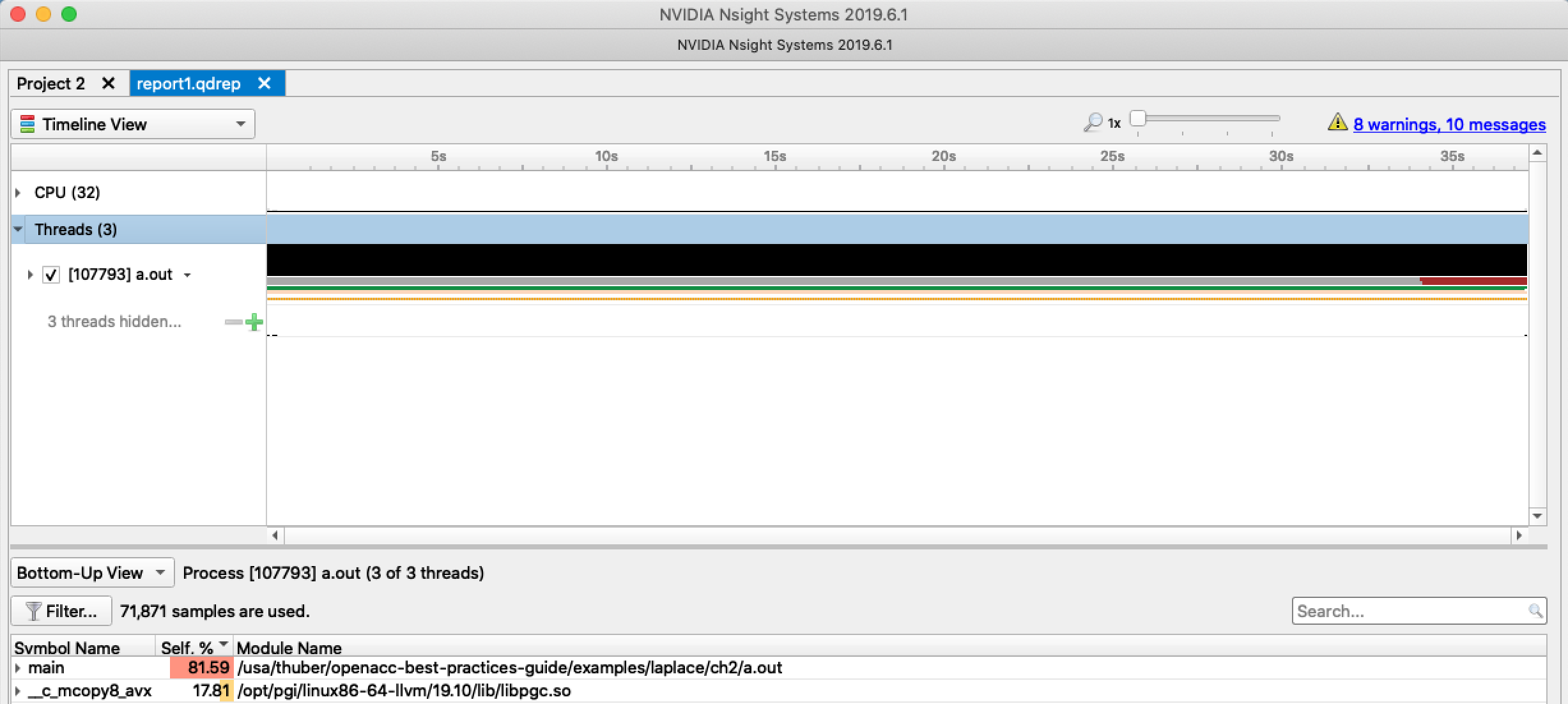
Clicking into the main function we can see that nearly all of the runtime within main comes from the loop that calculates the next value for A. This is shown in figure 2.2. What is not obvious from the profiler output, however, is that the time spent in the memory copy routine shown in the initial screen is actually the second loop nest, which performs the array swap at the end of each iteration. The compiler output shows above that the loop at line 68 was replaced by a memory copy, because doing so is more efficient than copying each element individually. So what the profiler is really showing us is that the major hotspots for our application are the loop nest that calculate Anew from A and the loop nest that copies from Anew to A for the next iteration, so we’ll concentrate our efforts on these two loop nests.

In the chapters that follow, we will optimize the loops identified in this chapter as the hotspots within our example application.