Advanced OpenACC Features
This chapter will discuss OpenACC features and techniques that do not fit neatly into other sections of the guide. These techniques are considered advanced, so readers should feel comfortable with the features discussed in previous chapters before proceeding to this chapter.
Asynchronous Operation
In a previous chapter we discussed the necessity to optimize for data locality
to reduce the cost of data transfers on systems where the host and accelerator
have physically distinct memories. There will always be some amount of data
transfers that simply cannot be optimized away and still produce correct
results. After minimizing data transfers, it may be possible to further reduce
the performance penalty associated with those transfers by overlapping the
copies with other operations on the host, device, or both. This can be achieved
with OpenACC using the async clause. The async clause can be added to
parallel, kernels, and update directives to specify that once the
associated operation has been sent to the accelerator or runtime for execution
the CPU may continue doing other things, rather than waiting for the
accelerator operation to complete. This may include enqueing additional
accelerator operations or computing other work that is unrelated to the work
being performed by the accelerator. The code below demonstrates adding the
async clause to a parallel loop and an update directive that follows.
    #pragma acc parallel loop async
    for (int i=0; i<N; i++)
    {
      c[i] = a[i] + b[i]
    }
    #pragma acc update self(c[0:N]) async
    !$acc parallel loop async
    do i=1,N
      c(i) = a(i) + b(i)
    end do
    !$acc update self(c) async
In the case above, the host thread will enqueue the parallel region into the
default asynchronous queue, then execution will return to the host thread so
that it can also enqueue the update, and finally the CPU thread will continue
execution. Eventually, however, the host thread will need the results computed
on the accelerator and copied back to the host using the update, so it must
synchronize with the accelerator to ensure that these operations have finished
before attempting to use the data. The wait directive instructs the runtime
to wait for past asynchronous operations to complete before proceeding. So, the
above examples can be extended to include a synchronization before the data
being copied by the update directive proceeds.
    #pragma acc parallel loop async
    for (int i=0; i<N; i++)
    {
      c[i] = a[i] + b[i]
    }
    #pragma acc update self(c[0:N]) async
    #pragma acc wait
    !$acc parallel loop async
    do i=1,N
      c(i) = a(i) + b(i)
    end do
    !$acc update self(c) async
    !$acc wait
While this is useful, it would be even more useful to expose dependencies into
these asynchronous operations and the associated waits such that independent
operations could potentially be executed concurrently. Both async and wait
have an optional argument for a non-negative, integer number that specifies a
queue number for that operation. All operations placed in the same queue will
operate in-order, but operations placed in different queues may operate in any
order with respect to each other. Operations in different queues may, but
are not guaranteed to, operate in parallel. These work queues are unique
per-device, so two devices will have distinct queues with the same number. If
a wait is encountered without an argument, it will wait on all previously
enqueued work on that device. The case study below will demonstrate how to
use different work queues to achieve overlapping of computation and data
transfers.
In addition to being able to place operations in separate queues, it’d be
useful to be able to join these queues together at a point where results from
both are needed before proceeding. This can be achieved by adding an async
clause to an wait. This may seem unintuitive, so the code below demonstrates
how this is done.
    #pragma acc parallel loop async(1)
    for (int i=0; i<N; i++)
    {
      a[i] = i;
    }
    #pragma acc parallel loop async(2)
    for (int i=0; i<N; i++)
    {
      b[i] = 2*i;
    }
    #pragma acc wait(1) async(2)
    #pragma acc parallel loop async(2)
    for (int i=0; i<N; i++)
    {
      c[i] = a[i] + b[i]
    }
    #pragma acc update self(c[0:N]) async(2)
    #pragma acc wait
    !$acc parallel loop async(1)
    do i=1,N
      a(i) = i
    end do
    !$acc parallel loop async(2)
    do i=1,N
      b(i) = 2.0 * i
    end do
    !$acc wait(1) async(2)
    !$acc parallel loop async(2)
    do i=1,N
      c(i) = a(i) + b(i)
    end do
    !$acc update self(c) async(2)
    !$acc wait
The above code initializes the values contained in a and b using separate
work queues so that they may potentially be done independently. The wait(1) async(2) ensures that work queue 2 does not proceed until queue 1 has
completed. The vector addition is then able to be enqueued to the device
because the previous kernels will have completed prior to this point. Lastly
the code waits for all previous operations to complete. Using this technique
we’ve expressed the dependencies of our loops to maximize concurrency between
regions but still give correct results.
Best Practice: The cost of sending an operation to the accelerator for
execution is frequently quite high on offloading accelerators, such as GPUs
connected over a PCIe bus to a host CPU. Once the loops and data transfers
within a routine have been tested, it is frequently beneficial to make each
parallel region and update asynchrounous and then place a wait directive
after the last accelerator directive. This allows the runtime to enqueue all of
the work immediately, which will reduce how often the accelerator and host must
synchronize and reduce the cost of launching work onto the accelerator. It is
criticial when implementing this optimization that the developer not leave off
the wait after the last accelerator directive, otherwise the code will be
likely to produce incorrect results. This is such a beneficial optimization
that some compilers provide a build-time option to enable this for all
accelerator directives automatically.
Case Study: Asynchronous Pipelining of a Mandelbrot Set

For this example we will be modifying a simple application that generates a
mandelbrot set, such as the picture shown above. Since each pixel of the image
can be independently calculated, the code is trivial to parallelize, but
because of the large size of the image itself, the data transfer to copy the
results back to the host before writing to an image file is costly. Since this
data transfer must occur, it’d be nice to overlap it with the computation, but
as the code is written below, the entire computation must occur before the copy
can occur, therefore there is noting to overlap. (Note: The mandelbrot
function is a sequential function used to calculate the value of each pixel. It
is left out of this chapter to save space, but is included in the full
examples.)
    #pragma acc parallel loop
    for(int y=0;y<HEIGHT;y++) {
      for(int x=0;x<WIDTH;x++) {
        image[y*WIDTH+x]=mandelbrot(x,y);
      }
    }

    #pragma acc update self(image[:WIDTH*HEIGHT])
    !$acc parallel loop
    do iy=1,width
      do ix=1,HEIGHT
        image(ix,iy) = min(max(int(mandelbrot(ix-1,iy-1)),0),MAXCOLORS)
      enddo
    enddo

    !$acc update self(image)
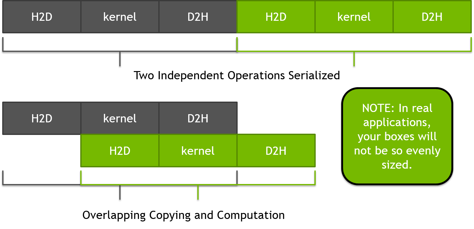
Since each pixel is independent of each other, it’s possible to use a technique known as pipelining to break up the generation of the image into smaller parts, which allows the output from each part to be copied while the next part is being computed. The figure below demonstrates an idealized pipeline where the computation and copies are equally sized, but this rarely occurs in real applications. By breaking the operation into two parts, the same amount of data is transferred, but all but the first and last transfers can be overlapped with computation. The number and size of these smaller chunks of work can be adjusted to find the value that provides the best performance.
The mandelbrot code can use this same technique by chunking up the image generation and data transfers into smaller, independent pieces. This will be done in multiple steps to reduce the likelihood of introducing an error. The first step is to introduce a blocking loop to the calculation, but keep the data transfers the same. This will ensure that the work itself is properly divided to give correct results. After each step the developer should build and run the code to ensure the resulting image is still correct.
Step 1: Blocking Computation
The first step in pipelining the image generation is to introduce a loop that
will break the computation up into chunks of work that can be generated
independently. To do this, we will need decide how many blocks of work is
desired and use that to determine the starting and ending bounds for each
block. Next we introduce an additional loop around the existing two and
modify the y loop to only operate within the current block of work by
updating its loop bounds with what we’ve calculated as the starting and ending
values for the current block. The modified loop nests are shown below.
    int num_blocks = 8;
    for(int block = 0; block < num_blocks; block++ ) {
      int ystart = block * (HEIGHT/num_blocks),
          yend   = ystart + (HEIGHT/num_blocks);
    #pragma acc parallel loop
      for(int y=ystart;y<yend;y++) {
        for(int x=0;x<WIDTH;x++) {
          image[y*WIDTH+x]=mandelbrot(x,y);
        }
      }
    }

    #pragma acc update self(image[:WIDTH*HEIGHT])
    num_batches=8
    batch_size=WIDTH/num_batches
    do yp=0,num_batches-1
      ystart = yp * batch_size + 1
      yend   = ystart + batch_size - 1
      !$acc parallel loop
      do iy=ystart,yend
        do ix=1,HEIGHT
          image(ix,iy) = min(max(int(mandelbrot(ix-1,iy-1)),0),MAXCOLORS)
        enddo
      enddo
    enddo

    !$acc update self(image)
At this point we have only confirmed that we can successfully generate each block of work independently. The performance of this step should not be noticably better than the original code and may be worse.
Step 2: Blocking Data Transfers
The next step in the process is to break up the data transfers to and from the
device in the same way the computation has already been broken up. To do this
we will first need to introduce a data region around the blocking loop. This
will ensure that the device memory used to hold the image will remain on the
device for all blocks of work. Since the initial value of the image array isn’t
important, we use a create data clause to allocate an uninitialized array on
the device. Next we use the update directive to copy each block of the image
from the device to the host after it has been calculated. In order to do this,
we need to determine the size of each block to ensure that we update only the
part of the image that coincides with the current block of work. The resulting
code at the end of this step is below.
    int num_blocks = 8, block_size = (HEIGHT/num_blocks)*WIDTH;
    #pragma acc data create(image[WIDTH*HEIGHT])
    for(int block = 0; block < num_blocks; block++ ) {
      int ystart = block * (HEIGHT/num_blocks),
          yend   = ystart + (HEIGHT/num_blocks);
    #pragma acc parallel loop
      for(int y=ystart;y<yend;y++) {
        for(int x=0;x<WIDTH;x++) {
          image[y*WIDTH+x]=mandelbrot(x,y);
        }
      }
    #pragma acc update self(image[block*block_size:block_size])
    }
    num_batches=8
    batch_size=WIDTH/num_batches
    call cpu_time(startt)
    !$acc data create(image)
    do yp=0,NUM_BATCHES-1
      ystart = yp * batch_size + 1
      yend   = ystart + batch_size - 1
      !$acc parallel loop
      do iy=ystart,yend
        do ix=1,HEIGHT
          image(ix,iy) = mandelbrot(ix-1,iy-1)
        enddo
      enddo
      !$acc update self(image(:,ystart:yend))
    enddo
    !$acc end data
By the end of this step we are calculating and copying each block of the image independently, but this is still being done sequentially, each block after the previous. The performance at the end of this step is generally comparable to the original version.
Step 3: Overlapping Computation and Transfers
The last step of this case study is to make the device operations asynchronous
so that the independent copies and computation can happen simultaneously.
To do this we will use asynchronous work queues to ensure that the computation
and data transfer within a single block are in the same queue, but separate
blocks land in different queues. The block number is a convenient asynchronous
handle to use for this change. Of course, since we’re now operating completely
asynchronously, it’s critical that we add a wait directive after the block loop
to ensure that all work completes before we attempt to use the image data from
the host. The modified code is found below.
    int num_blocks = 8, block_size = (HEIGHT/num_blocks)*WIDTH;
    #pragma acc data create(image[WIDTH*HEIGHT])
    for(int block = 0; block < num_blocks; block++ ) {
      int ystart = block * (HEIGHT/num_blocks),
          yend   = ystart + (HEIGHT/num_blocks);
    #pragma acc parallel loop async(block)
      for(int y=ystart;y<yend;y++) {
        for(int x=0;x<WIDTH;x++) {
          image[y*WIDTH+x]=mandelbrot(x,y);
        }
      }
    #pragma acc update self(image[block*block_size:block_size]) async(block)
    }
    #pragma acc wait
    num_batches=8
    batch_size=WIDTH/num_batches
    call cpu_time(startt)
    !$acc data create(image)
    do yp=0,NUM_BATCHES-1
      ystart = yp * batch_size + 1
      yend   = ystart + batch_size - 1
      !$acc parallel loop async(yp)
      do iy=ystart,yend
        do ix=1,HEIGHT
          image(ix,iy) = mandelbrot(ix-1,iy-1)
        enddo
      enddo
      !$acc update self(image(:,ystart:yend)) async(yp)
    enddo
    !$acc wait
    !$acc end data
With this modification it’s now possible for the computational part of one block to operate simultaneously as the data transfer of another. The developer should now experiment with varying block sizes to determine what the optimal value is on the architecture of interest. It’s important to note, however, that on some architectures the cost of creating an asynchronous queue the first time its used can be quite expensive. In long-running applications, where the queues may be created once at the beginning of a many-hour run and reused throughout, this cost is amortized. In short-running codes, such as the demonstration code used in this chapter, this cost may outweigh the benefit of the pipelining. Two solutions to this are to introduce a simple block loop at the beginning of the code that pre-creates the asynchronous queues before the timed section, or to use a modulus operation to reuse the same smaller number of queues among all of the blocks. For instance, by using the block number modulus 2 as the asynchronous handle, only two queues will be used and the cost of creating those queues will be amortized by their reuse. Two queues is generally sufficient to see a gain in performance, since it still allows computation and updates to overlap, but the developer should experiment to find the best value on a given machine.
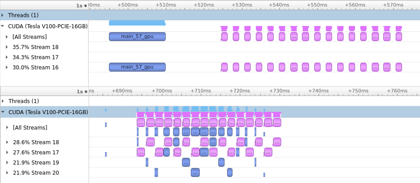
Below we see a screenshot showing before and after profiles from applying these changes to the code on an NVIDIA GPU platform. Similar results should be possible on any acclerated platform. Using 16 blocks and two asynchronous queues, as shown below, roughly a 2X performance improvement was observed on the test machine over the performance without pipelining.
Multi-device Programming
For systems containing more than one accelerator, OpenACC provides an API to make operations happen on a particular device. In case a system contains accelerators of different types, the specification also allows for querying and selecting devices of a specific architecture.
acc_get_num_devices()
The acc_get_num_devices() routine may be used to query how many devices of
a given architecture are available on the system. It accepts one parameter of
type acc_device_t and returns a integer number of devices.
acc_get_device_num() and acc_set_device_num()
The acc_get_device_num() routines query the
current device that will be used of a given type and returns the integer
identifier of that device. The acc_set_device_num() accepts two parameters,
the desired device number and device type. Once a device number has been set,
all operations will be sent to the specified device until a different device
is specified by a later call to acc_set_device_num().
acc_get_device_type() and acc_set_device_type()
The acc_get_device_type() routine takes no parameters and returns the device
type of the current default device. The acc_set_device_type() specifies to
the runtime the type of device that the runtime should use for accelerator
operations, but allows the runtime to choose which device of that type to use.
OpenACC has recently introduced the set directive, which allows for
multi-device programming with less reliance on using the OpenACC API.
The set directive can be used to set the device number and device type
that should be used and is functionally equivalent to the
acc_set_device_num() API function. To set the device number, use
device_num clause, and to set the type use the device_type clause.
Multi-device Programming Example
As an example of multi-device programming, it’s possible to further extend the
mandelbrot example used previously to send different blocks of work to
different accelerators. In order to make this work, it’s necessary to ensure
that device copies of the data are created on each device. We will do this by
replacing the structured data region in the code with an unstructured enter data
directive for each device, using the acc_set_device_num() function to
specify the device for each enter data. For simplicity, we will allocate the
full image array on each device, although only a part of the array is actually
needed. When the memory requirements of the application is large, it will be
necessary to allocate just the pertinent parts of the data on each accelerator.
Once the data has been created on each device, a call to acc_set_device_num()
in the blocking loop, using a simple modulus operation to select which device
should receive each block, will send blocks to different devices.
Lastly it’s necessary to introduce a loop over devices to wait on each device
to complete. Since the wait directive is per-device, the loop will once again
use acc_set_device_num() to select a device to wait on, and then use an
exit data directive to deallocate the device memory. The final code is below.
    // Allocate arrays on both devices
    for (int gpu=0; gpu < 2 ; gpu ++)
    {
      acc_set_device_num(gpu,acc_device_nvidia);
    #pragma acc enter data create(image[:bytes])
    }

    // Distribute blocks between devices
    for(int block=0; block < numblocks; block++)
    {
      int ystart = block * blocksize;
      int yend   = ystart + blocksize;
      acc_set_device_num(block%2,acc_device_nvidia);
    #pragma acc parallel loop async(block)
      for(int y=ystart;y<yend;y++) {
        for(int x=0;x<WIDTH;x++) {
          image[y*WIDTH+x]=mandelbrot(x,y);
        }
      }
    #pragma acc update self(image[ystart*WIDTH:WIDTH*blocksize]) async(block)
    }

    // Wait on each device to complete and then deallocate arrays
    for (int gpu=0; gpu < 2 ; gpu ++)
    {
      acc_set_device_num(gpu,acc_device_nvidia);
    #pragma acc wait
    #pragma acc exit data delete(image)
    }
    batch_size=WIDTH/num_batches
    do gpu=0,1
      call acc_set_device_num(gpu,acc_device_nvidia)
      !$acc enter data create(image)
    enddo
    do yp=0,NUM_BATCHES-1
      call acc_set_device_num(mod(yp,2),acc_device_nvidia)
      ystart = yp * batch_size + 1
      yend   = ystart + batch_size - 1
      !$acc parallel loop async(yp)
      do iy=ystart,yend
        do ix=1,HEIGHT
          image(ix,iy) = mandelbrot(ix-1,iy-1)
        enddo
      enddo
      !$acc update self(image(:,ystart:yend)) async(yp)
    enddo
    do gpu=0,1
      call acc_set_device_num(gpu,acc_device_nvidia)
      !$acc wait
      !$acc exit data delete(image)
    enddo
Although this example over-allocates device memory by placing the entire image array
on the device, it does serve as a simple example of how the acc_set_device_num()
routine can be used to operate on a machine with multiple devices. In
production codes the developer will likely want to partition the work such that
only the parts of the array needed by a specific device are available there.
Additionally, by using CPU threads it may be possible to issue work to the
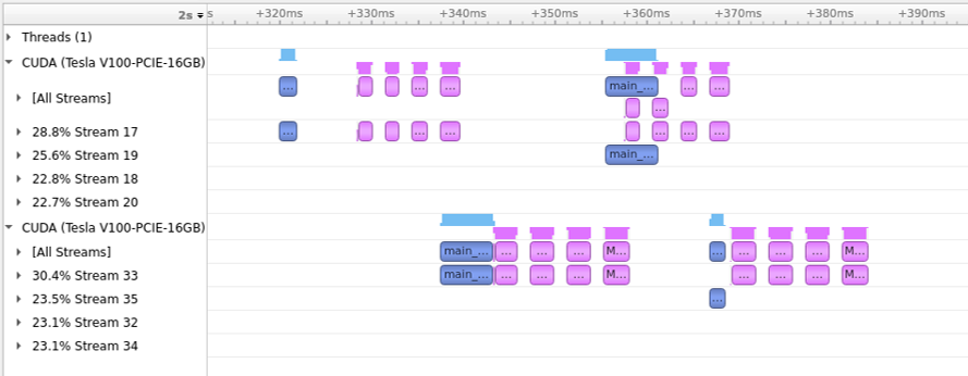
devices more quickly and improve overall performance. Figure 7.3
shows a screenshot of the NVIDIA NSight Systems showing the mandelbrot
computation divided across two NVIDIA GPUs.