Optimize Loops
Once data locality has been expressed, developers may wish to further tune the code for the hardware of interest. It’s important to understand that the more loops are tuned for a particular type of hardware the less performance portable the code becomes to other architectures. If you’re generally running on one particular accelerator, however, there may be some gains to be had by tuning how the loops are mapped to the underlying hardware.
It’s tempting to begin tuning the loops before all of the data locality has been expressed in the code. However, because data copies are frequently the limiter to application performance on the current generation of accelerators the performance impact of tuning a particular loop may be too difficult to measure until data locality has been optimized. For this reason the best practice is to wait to optimize particular loops until after all of the data locality has been expressed in the code, reducing the data transfer time to a minimum.
Efficient Loop Ordering
Before changing the way OpenACC maps loops onto the hardware of interest, the developer should examine the important loops to ensure that data arrays are being accessed in an efficient manner. Most modern hardware, be it a CPU with large caches and SIMD operations or a GPU with coalesced memory accesses and SIMT operations, favor accessing arrays in a stride 1 manner. That is to say that each loop iteration accesses consecutive memory addresses. This is achieved by ensuring that the innermost loop of a loop nest iterates on the fastest varying array dimension and each successive loop outward accesses the next fastest varying dimension. Arranging loops in this increasing manner will frequently improve cache efficiency and improve vectorization on most architectures.
OpenACC’s 3 Levels of Parallelism
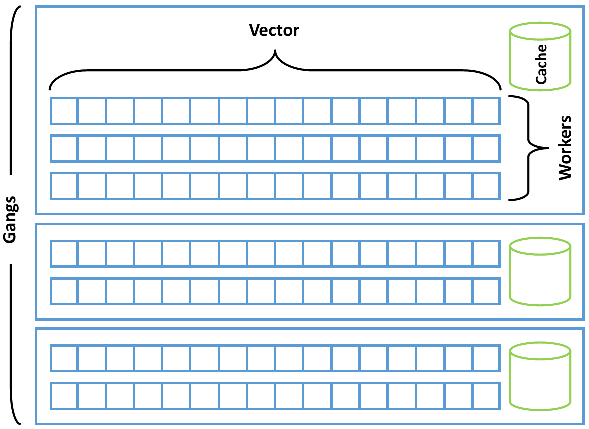
OpenACC defines three levels of parallelism: gang, worker, and vector. Additionally execution may be marked as being sequential (seq). Vector parallelism has the finest granularity, with an individual instruction operating on multiple pieces of data (much like SIMD parallelism on a modern CPU or SIMT parallelism on a modern GPU). Vector operations are performed with a particular vector length, indicating how many data elements may be operated on with the same instruction. Gang parallelism is coarse-grained parallelism, where gangs work independently of each other and may not synchronize. Worker parallelism sits between vector and gang levels. A gang consists of 1 or more workers, each of which operates on a vector of some length. Within a gang the OpenACC model exposes a cache memory, which can be used by all workers and vectors within the gang, and it is legal to synchronize within a gang, although OpenACC does not expose synchronization to the user. Using these three levels of parallelism, plus sequential, a programmer can map the parallelism in the code to any device. OpenACC does not require the programmer to do this mapping explicitly, however. If the programmer chooses not to explicitly map loops to the device of interest the compiler will implicitly perform this mapping using what it knows about the target device. This makes OpenACC highly portable, since the same code may be mapped to any number of target devices. The more explicit mapping of parallelism the programmer adds to the code, however, the less portable they make the code to other architectures.
Understanding OpenACC’s Three Levels of Parallelism
The terms gang, worker, and vector are foreign to most programmers, so the meanings of these three levels of parallelism is often lost on new OpenACC programmers. Here’s a practical example to help understand these three levels. Imagine that you need to paint your apartment. One person with a roller and bucket of paint can be reasonably expected to paint a small apartment in a few hours, maybe a day. For a small apartment, one painter is probably enough to complete the job, but what about if I need to paint every apartment in a large, multi-story building. In that case, it’s a pretty daunting task for one person to complete. There’s a few tricks this painter may try in order to work more quickly. One option is to work faster, moving the roller across the wall as fast that their arm can manage. There’s a practical limit, however, to how fast a human being can actually use a paint roller. Another option is to use a larger paint roller. Perhaps our painter started with a 4 inch paint roller, so if they upgraded to an 8 inch roller, they can cover twice as much wall space in the same amount of time. Why stop there? Let’s buy a 32 inch paint roller to cover even more wall per stroke! Now we’re going to start to run into different problems. For instance, the painter’s arm probably can’t move as fast with a 32 inch roller as an 8 inch, so there’s no guarantee that this is actually faster. Futhermore, wider rollers may result in awkward times when the painter has to paint over a place they’ve already painted just so that the roller fits or the wider roller may take more time to fill with paint. In either case, there’s a clear limit to how fast a single painter can get the job done, so let’s invite more painters.
Now assume I have 4 painters working on the job. If given independent areas to paint, the job should get gone nearly 4 times faster, but at the cost of getting 4 times as many rollers, paint pans, and cans of paint. This is probably a small price to pay to get the job done nearly 4 times faster. Large jobs require large crews, however, so let’s increase the number of painters again to 16. If each painter can work independently then the time it takes to complete the painting will probably go down by another 4 times, but now there may be some other inefficencies. For instance, it’s probably cheaper to buy large buckets of the paint, rather than small paint cans, so we’ll store those buckets in a central location where everyone can access them. Now if a painter needs to refill their can, they have to walk to get their paint, which takes away from the time they’re painting. Here’s an idea, let’s organize our 16 painters into 4 groups of 4 painters, each of which has their own bucket to share. Now so long as the painters within each crew is working on jobs near the rest of the crew, the walk to get more paint is much shorter, but the crews are still free to work completely independently of each other.
In this analogy, there’s 3 levels of parallelism, just like OpenACC. The finest-grained level may not be completely obvious, but it’s the size of the roller. The width of the roller dictates how much wall the painter can paint with each stroke. Wider rollers mean more wall per stroke, up to some limit. Next there are parallel painters within each crew. These painters can work mostly independently of each other, but occasionally need to access their shared paint bucket or coordinate the next, near-by piece of work to do. Finally, there’s our crews, which can work completely independently of each other and might even work at different times (think, day shift and night shift), representing the coarsest-grained parallelism in our hierarchy.
In OpenACC gangs are like the work crews, they are completely independent of each other and may operate in parallel or even at different times. Workers are the individual painters, they can operate on their own but may also share resources with other workers in the same gang. Finally the paint roller represents the vector where the width of the roller represents the vector length. Workers perform the same instruction on multiple elements of data using vector operations. So, gangs consist of at least one worker, which operates on a vector of data.
Mapping Parallelism to the Hardware
With some understanding of how the underlying accelerator hardware works it’s possible to inform the compiler how it should map the loop iterations into parallelism on the hardware. It’s worth restating that the more detail the compiler is given about how to map the parallelism onto a particular accelerator the less performance portable the code will be. For instance, setting a fixed vector length may enhance performance on one processor and hinder performance on another or fixing the number of gangs used to execute on a loop may result in limiting the performance on processors with a larger degree of parallelism.
As discussed earlier in this guide, the loop directive is intended to give the
compiler additional information about the next loop in the code. In addition to
the clauses shown before, which were intended to ensure correctness, the
clauses below inform the compiler which level of parallelism should be used to
for the given loop.
Gang clause - partition the loop across gangs
Worker clause - partition the loop across workers
Vector clause - vectorize the loop
Seq clause - do not partition this loop, run it sequentially instead
These directives may also be combined on a particular loop. For example, a
gang vector loop would be partitioned across gangs, each of which with 1
worker implicitly, and then vectorized. The OpenACC specification enforces that
the outermost loop must be a gang loop, the innermost parallel loop must be
a vector loop, and a worker loop may appear in between. A sequential loop may
appear at any level.
    #pragma acc parallel loop gang
    for ( i=0; i<N; i++)
      #pragma acc loop vector
      for ( j=0; j<M; j++)
        ;
–
    !$acc parallel loop gang
    do j=1,M
      !$acc loop vector
      do i=1,N
Informing the compiler where to partition the loops is just one part of
optimizing the loops. The programmer may additionally tell the compiler the
specific number of gangs, workers, or the vector length to use for the loops.
This specific mapping is achieved slightly differently when using the kernels
directive or the parallel directive. In the case of the kernels directive,
the gang, worker, and vector clauses accept an integer parameter that
will optionally inform the compiler how to partition that level of parallelism.
For example, vector(128) informs the compiler to use a vector length of 128
for the loop.
    #pragma acc kernels
    {
    #pragma acc loop gang
    for ( i=0; i<N; i++)
      #pragma acc loop vector(128)
      for ( j=0; j<M; j++)
        ;
    }
    !$acc kernels
    !$acc loop gang
    do j=1,M
      !$acc loop vector(128)
      do i=1,N

    !$acc end kernels
When using the parallel directive, the information is presented
on the parallel directive itself, rather than on each individual loop, in the
form of the num_gangs, num_workers, and vector_length clauses to the
parallel directive.
    #pragma acc parallel loop gang vector_length(128)
    for ( i=0; i<N; i++)
      #pragma acc loop vector
      for ( j=0; j<M; j++)
        ;
    !$acc parallel loop gang vector_length(128)
    do j=1,M
      !$acc loop vector
      do i=1,N
Since these mappings will vary between different accelerator, the loop
directive accepts a device_type clause, which will inform the compiler that
these clauses only apply to a particular device type. Clauses after a
device_type clause up until either the next device_type or the end of the
directive will apply only to the specified device. Clauses that appear before
all device_type clauses are considered default values, which will be used if
they are not overridden by a later clause. For example, the code below
specifies that a vector length of 128 should be used on devices of type
acc_device_nvidia or a vector length of 256 should be used on devices of
type acc_device_radeon. The compiler will choose a default vector length for
all other device types.
    #pragma acc parallel loop gang vector \
                device_type(acc_device_nvidia) vector_length(128) \
                device_type(acc_device_radeon) vector_length(256)
    for (i=0; i<N; i++)
    {
      y[i] = 2.0f * x[i] + y[i];
    }
Collapse Clause
When a code contains tightly nested loops it is frequently beneficial to collapse these loops into a single loop. Collapsing loops means that two loops of trip counts N and M respectively will be automatically turned into a single loop with a trip count of N times M. By collapsing two or more parallel loops into a single loop the compiler has an increased amount of parallelism to use when mapping the code to the device. On highly parallel architectures, such as GPUs, this can result in improved performance. Additionally, if a loop lacked sufficient parallelism for the hardware by itself, collapsing it with another loop multiplies the available parallelism. This is especially beneficial on vector loops, since some hardware types will require longer vector lengths to achieve high performance than others. Collapsing gang loops may also be beneficial if it allows for generating a greater number of gangs for highly-parallel processors. The code below demonstrates how to use the collapse directive.
    #pragma acc parallel loop gang collapse(2)
    for(ie = 0; ie < nelemd; ie++) {
      for(q = 0; q < qsize; q++) {
        #pragma acc loop vector collapse(3)
        for(k = 0; k < nlev; k++) {
          for(j = 0; j < np; j++) {
            for(i = 0; i < np; i++) {
              qtmp = elem[ie].state.qdp[i][j][k][q][n0_qdp];
              vs1tmp = vstar[i][j][k][0][ie] * elem[ie].metdet[i][j] * qtmp;
              vs2tmp = vstar[i][j][k][1][ie] * elem[ie].metdet[i]]j] * qtmp;
              gv[i][j][k][0] = (dinv[i][j][0][0][ie] * vs1tmp + dinv[i][j][0][1][ie] * vs2tmp);
              gv[i][j][k][1] = (dinv[i][j][1][0][ie] * vs1tmp + dinv[i][j][1][1][ie] * vs2tmp);
            }
          }
        }
      }
    }
    ! $acc parallel loop gang collapse (2)
    do ie = 1 , nelemd
      do q = 1 , qsize
        ! $acc loop vector collapse (3)
        do k = 1 , nlev
          do j = 1 , np
            do i = 1 , np
              qtmp = elem (ie )% state % qdp (i,j,k,q, n0_qdp )
              vs1tmp = vstar (i,j,k ,1, ie) * elem (ie )% metdet (i,j) * qtmp
              vs2tmp = vstar (i,j,k ,2, ie) * elem (ie )% metdet (i,j) * qtmp
              gv(i,j,k ,1) = ( dinv (i,j ,1 ,1 , ie )* vs1tmp + dinv (i,j ,1 ,2, ie )* vs2tmp )
              gv(i,j,k ,2) = ( dinv (i,j ,2 ,1 , ie )* vs1tmp + dinv (i,j ,2 ,2, ie )* vs2tmp )
            enddo
          enddo
        enddo
      enddo
    enddo
The above code is an excerpt from a real application where collapsing loops
extended the parallelism available to be exploited. On line 1, the two
outermost loops are collapsed together to make it possible to generate gangs
across the iterations of both loops, thus making the possible number of gangs
nelemd x qsize rather than just nelemd. The collapse at line 4 collapses
together 3 small loops to increase the possible vector length, as none of the
loops iterate for enough trips to create a reasonable vector length on the
target accelerator. How much this optimization will speed-up the code will vary
according to the application and the target accelerator, but it’s not uncommon
to see large speed-ups by using collapse on loop nests.
Routine Parallelism
A previous chapter introduced the routine directive for calling functions and
subroutines from OpenACC parallel regions. In that chapter it was assumed that
the routine would be called from each loop iteration, therefore requiring a
routine seq directive. In some cases, the routine itself may contain
parallelism that must be mapped to the device. In these cases, the routine
directive may have a gang, worker, or vector clause instead of seq to
inform the compiler that the routine will contain the specified level of
parallelism. This can be thought of as reserving a particular level of
parallelism for the loops in that routine. This is so that when the compiler
then encounters the call site of the affected routine, it will then know how
it can parallelize the code to use the routine. It’s important to note that
if an acc routine calls another routine, that routine must also have an
acc routine directive. At this time the OpenACC specification does not
allow for specifying multiple possible levels of parallelism on a single
routine.
Case Study - Optimize Loops
This case study will focus on a different algorithm than the previous chapters. When a compiler has sufficient information about loops to make informed decisions, it’s frequently difficult to improve the performance of a given parallel loop by more than a few percent. In some cases, the code lacks the information necessary for the compiler to make informed optimization decisions. In these cases, it’s often possible for a developer to optimize the parallel loops significantly by informing the compiler how to decompose and distribute the loops to the hardware.
The code used in this section implements a sparse, matrix-vector product (SpMV) operation. This means that a matrix and a vector will be multiplied together, but the matrix has very few elements that are not zero (it is sparse), meaning that calculating these values is unnecessary. The matrix is stored in a Compress Sparse Row (CSR) format. In CSR the sparse array, which may contain a significant number of cells whose value is zero, thus wasting a significant amount of memory, is stored using three, smaller arrays: one containing the non-zero values from the matrix, a second that describes where in a given row these non-zero elements would reside, and a third describing the columns in which the data would reside. The code for this exercise is below.
    #pragma acc parallel loop
    for(int i=0;i<num_rows;i++) {
      double sum=0;
      int row_start=row_offsets[i];
      int row_end=row_offsets[i+1];
      #pragma acc loop reduction(+:sum)
      for(int j=row_start;j<row_end;j++) {
        unsigned int Acol=cols[j];
        double Acoef=Acoefs[j];
        double xcoef=xcoefs[Acol];
        sum+=Acoef*xcoef;
      }
      ycoefs[i]=sum;
    }
    !$acc parallel loop
    do i=1,a%num_rows
      tmpsum = 0.0d0
      row_start = arow_offsets(i)
      row_end   = arow_offsets(i+1)-1
      !$acc loop reduction(+:tmpsum)
      do j=row_start,row_end
        acol = acols(j)
        acoef = acoefs(j)
        xcoef = x(acol)
        tmpsum = tmpsum + acoef*xcoef
      enddo
      y(i) = tmpsum
    enddo
One important thing to note about this code is that the compiler is unable to determine how many non-zeros each row will contain and use that information in order to schedule the loops. The developer knows, however, that the number of non-zero elements per row is very small and this detail will be key to achieving high performance.
NOTE: Because this case study features optimization techniques, it is necessary to perform optimizations that may be beneficial on one hardware, but not on others. This case study was performed using the NVHPC 20.11 compiler on an NVIDIA Volta V100 GPU. These same techniques may apply on other architectures, particularly those similar to NVIDIA GPUs, but it will be necessary to make certain optimization decisions based on the particular accelerator in use.
In examining the compiler feedback from the code shown below, I know that the compiler has chosen to use a vector length of 256 on the innermost loop. I could have also obtained this information from a runtime profile of the application.
    matvec(const matrix &, const vector &, const vector &):
          3, Generating Tesla code
              4, #pragma acc loop gang /* blockIdx.x */
              9, #pragma acc loop vector(256) /* threadIdx.x */
                 Generating reduction(+:sum)
          3, Generating present(ycoefs[:],xcoefs[:],row_offsets[:],Acoefs[:],cols[:])
          9, Loop is parallelizable
Based on my knowledge of the matrix, I know that this is significantly larger than the typical number of non-zeros per row, so many of the vector lanes on the accelerator will be wasted because there’s not sufficient work for them. The first thing to try in order to improve performance is to adjust the vector length used on the innermost loop. I happen to know that the compiler I’m using will restrict me to using multiples of the warp size (the minimum SIMT execution size on NVIDIA GPUs) of this processor, which is 32. This detail will vary according to the accelerator of choice. Below is the modified code using a vector length of 32.
    #pragma acc parallel loop vector_length(32)
    for(int i=0;i<num_rows;i++) {
      double sum=0;
      int row_start=row_offsets[i];
      int row_end=row_offsets[i+1];
      #pragma acc loop vector reduction(+:sum)
      for(int j=row_start;j<row_end;j++) {
        unsigned int Acol=cols[j];
        double Acoef=Acoefs[j];
        double xcoef=xcoefs[Acol];
        sum+=Acoef*xcoef;
      }
      ycoefs[i]=sum;
    }
    !$acc parallel loop vector_length(32)
    do i=1,a%num_rows
      tmpsum = 0.0d0
      row_start = arow_offsets(i)
      row_end   = arow_offsets(i+1)-1
      !$acc loop vector reduction(+:tmpsum)
      do j=row_start,row_end
        acol = acols(j)
        acoef = acoefs(j)
        xcoef = x(acol)
        tmpsum = tmpsum + acoef*xcoef
      enddo
      y(i) = tmpsum
    enddo
Notice that I have now explicitly informed the compiler that the innermost loop
should be a vector loop, to ensure that the compiler will map the parallelism
exactly how I wish. I can try different vector lengths to find the optimal
value for my accelerator by modifying the vector_length clause. Below is a graph
showing the relative speed-up of varying the vector length
compared to the compiler-selected value.
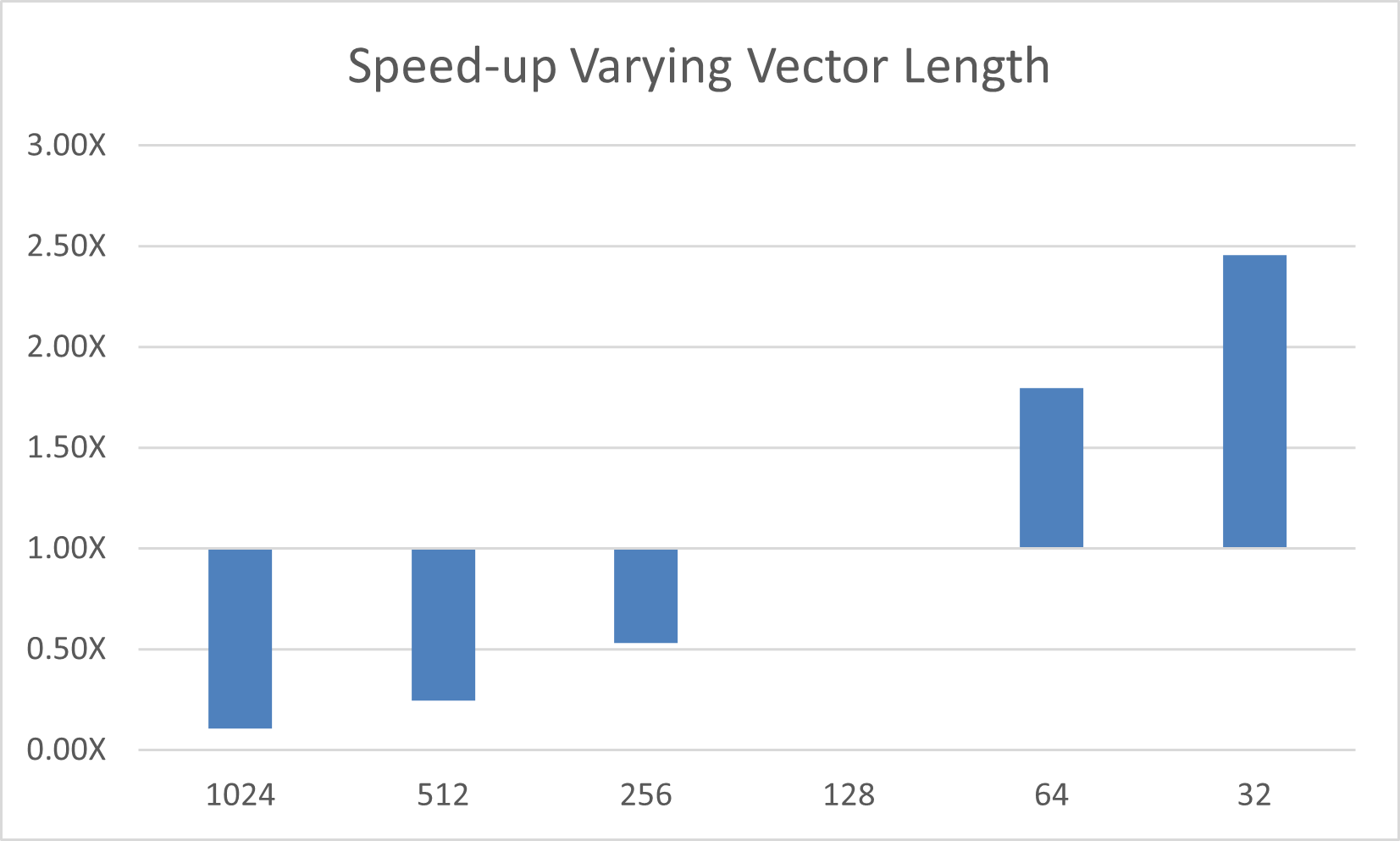
Notice that the best performance comes from the smallest vector length. Again, this is because the number of non-zeros per row is very small, so a small vector length results in fewer wasted compute resources. On the particular chip I’m using, the smallest possible vector length, 32, achieves the best possible performance. On this particular accelerator, I also know that the hardware will not perform efficiently at this vector length unless we can identify further parallelism another way. In this case, we can use the worker level of parallelism to fill each gang with more of these short vectors. Below is the modified code.
    #pragma acc parallel loop gang worker num_workers(4) vector_length(32)
    for(int i=0;i<num_rows;i++) {
      double sum=0;
      int row_start=row_offsets[i];
      int row_end=row_offsets[i+1];
      #pragma acc loop vector
      for(int j=row_start;j<row_end;j++) {
        unsigned int Acol=cols[j];
        double Acoef=Acoefs[j];
        double xcoef=xcoefs[Acol];
        sum+=Acoef*xcoef;
      }
      ycoefs[i]=sum;
    }
    !$acc parallel loop gang worker num_workers(32) vector_length(32)
    do i=1,a%num_rows
      tmpsum = 0.0d0
      row_start = arow_offsets(i)
      row_end   = arow_offsets(i+1)-1
      !$acc loop vector reduction(+:tmpsum)
      do j=row_start,row_end
        acol = acols(j)
        acoef = acoefs(j)
        xcoef = x(acol)
        tmpsum = tmpsum + acoef*xcoef
      enddo
      y(i) = tmpsum
    enddo
In this version of the code, I’ve explicitly mapped the outermost loop to both
gang and worker parallelism and will vary the number of workers using the
num_workers clause. The results follow.
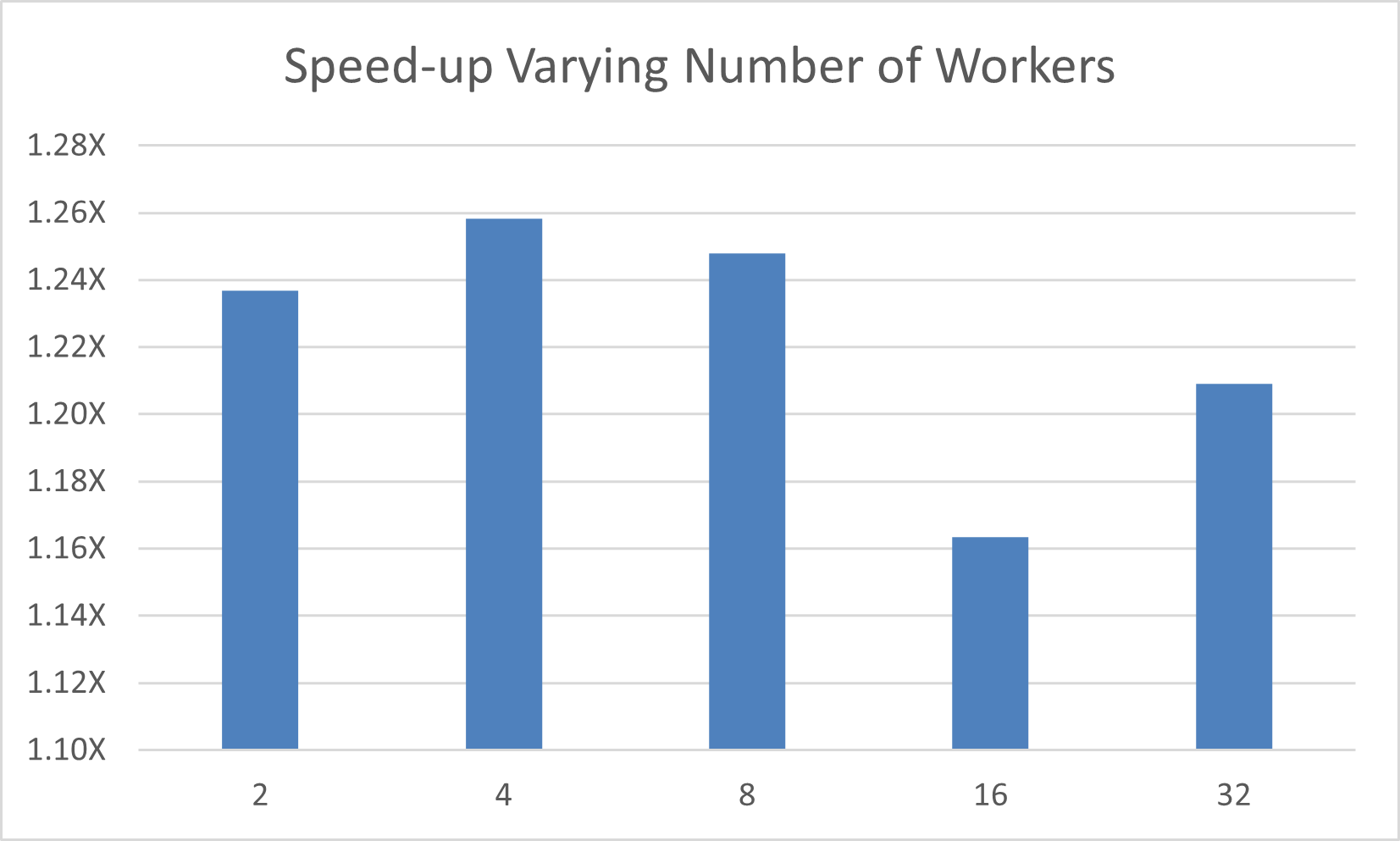
On this particular hardware, the best performance comes from a vector length of 32 and 4 workers, which is similar to the simpler loop with a default vector length of 128. In this case, we observed a 2.5X speed-up from decreasing the vector length and another 1.26X speed-up from varying the number of workers within each gang, resulting in an overall 3.15X performance improvement from the untuned OpenACC code.
Best Practice: Although not shown in order to save space, it’s generally
best to use the device_type clause whenever specifying the sorts of
optimizations demonstrated in this section, because these clauses will likely
differ from accelerator to accelerator. By using the device_type clause it’s
possible to provide this information only on accelerators where the
optimizations apply and allow the compiler to make its own decisions on other
architectures. The OpenACC specification specifically suggests nvidia,
radeon, and host as three common device type strings.