Parallelize Loops
Now that the important hotspots in the application have been identified, the programmer should incrementally accelerate these hotspots by adding OpenACC directives to the important loops within those routines. There is no reason to think about the movement of data at this point in the process, the OpenACC compiler will analyze the data needed in the identified region and automatically ensure that the data is available on the accelerator. By focusing solely on the parallelism during this step, the programmer can move as much computation to the device as possible and ensure that the program is still giving correct results before optimizing away data motion in the next step. During this step in the process it is common for the overall runtime of the application to increase, even if the execution of the individual loops is faster using the accelerator. This is because the compiler must take a cautious approach to data movement, frequently copying more data to and from the accelerator than is actually necessary. Even if overall execution time increases during this step, the developer should focus on expressing a significant amount of parallelism in the code before moving on to the next step and realizing a benefit from the directives.
OpenACC provides two different approaches for exposing parallelism in the code:
parallel and kernels regions. Each of these directives will be detailed in
the sections that follow.
The Kernels Construct
The kernels construct identifies a region of code that may contain
parallelism, but relies on the automatic parallelization capabilities of the
compiler to analyze the region, identify which loops are safe to parallelize,
and then accelerate those loops. Developers with little or no parallel
programming experience, or those working on functions containing many loop
nests that might be parallelized, will find the kernels directive a good
starting place for OpenACC acceleration. The code below demonstrates the use of
kernels in both C/C++ and Fortran.
    #pragma acc kernels
    {
      for (i=0; i<N; i++)
      {
        y[i] = 0.0f;
        x[i] = (float)(i+1);
      }

      for (i=0; i<N; i++)
      {
        y[i] = 2.0f * x[i] + y[i];
      }
    }
    !$acc kernels
    do i=1,N
      y(i) = 0
      x(i) = i
    enddo

    do i=1,N
      y(i) = 2.0 * x(i) + y(i)
    enddo
    !$acc end kernels
In this example the code is initializing two arrays and then performing a
simple calculation on them. Notice that we have identified a block of code,
using curly braces in C and starting and ending directives in Fortran, that
contains two candidate loops for acceleration. The compiler will analyze these
loops for data independence and parallelize both loops by generating an
accelerator kernel for each. The compiler is given complete freedom to
determine how best to map the parallelism available in these loops to the
hardware, meaning that we will be able to use this same code regardless of the
accelerator we are building for. The compiler will use its own knowledge of the
target accelerator to choose the best path for acceleration. One caution about
the kernels directive, however, is that if the compiler cannot be certain
that a loop is data independent, it will not parallelize the loop. Common
reasons for why a compiler may misidentify a loop as non-parallel will be
discussed in a later section.
The Parallel Construct
The parallel construct identifies a region of code that will be parallelized
across OpenACC gangs. By itself a parallel region is of limited use,
but when paired with the loop directive (discussed in more detail later) the
compiler will generate a parallel version of the loop for the accelerator.
These two directives can, and most often are, combined into a single parallel loop directive. By placing this directive on a loop the programmer asserts
that the affected loop is safe to parallelize and allows the compiler to select
how to schedule the loop iterations on the target accelerator. The code below
demonstrates the use of the parallel loop combined directive in both C/C++
and Fortran.
    #pragma acc parallel loop
      for (i=0; i<N; i++)
      {
        y[i] = 0.0f;
        x[i] = (float)(i+1);
      }

    #pragma acc parallel loop
      for (i=0; i<N; i++)
      {
        y[i] = 2.0f * x[i] + y[i];
      }
    !$acc parallel loop
    do i=1,N
      y(i) = 0
      x(i) = i
    enddo

    !$acc parallel loop
    do i=1,N
      y(i) = 2.0 * x(i) + y(i)
    enddo
Notice that, unlike the kernels directive, each loop needs to be explicitly
decorated with parallel loop directives. This is because the parallel
construct relies on the programmer to identify the parallelism in the code
rather than performing its own compiler analysis of the loops. In this case,
the programmer is only identifying the availability of parallelism, but still
leaving the decision of how to map that parallelism to the accelerator to the
compiler’s knowledge about the device. This is a key feature that
differentiates OpenACC from other similar programming models. The programmer
identifies the parallelism without dictating to the compiler how to exploit
that parallelism. This means that OpenACC code will be portable to devices
other than the device on which the code is being developed, because details
about how to parallelize the code are left to compiler knowledge rather than
being hard-coded into the source.
Differences Between Parallel and Kernels
One of the biggest points of confusion for new OpenACC programmers is why the
specification has both the parallel and kernels directives, which appear to
do the same thing. While they are very closely related there are subtle
differences between them. The kernels construct gives the compiler maximum
leeway to parallelize and optimize the code how it sees fit for the target
accelerator, but also relies most heavily on the compiler’s ability to
automatically parallelize the code. As a result, the programmer may see
differences in what different compilers are able to parallelize and how they do
so. The parallel loop directive is an assertion by the programmer
that it is both safe and desirable to parallelize the affected loop. This
relies on the programmer to have correctly identified parallelism in the code
and remove anything in the code that may be unsafe to parallelize. If the
programmer asserts incorrectly that the loop may be parallelized then the
resulting application may produce incorrect results.
To put things another way: the kernels construct may be thought of as a hint
to the compiler of where it should look for parallelism while the parallel
directive is an assertion to the compiler of where there is parallelism.
An important thing to note about the kernels construct is that the compiler
will analyze the code and only parallelize when it is certain that it is safe
to do so. In some cases the compiler may not have enough information at
compile time to determine whether a loop is safe to parallelize, in which case
it will not parallelize the loop, even if the programmer can clearly see that
the loop is safely parallel. For example, in the case of C/C++ code, where
arrays are represented as pointers, the compiler may not always be
able to determine that two arrays do not reference the same memory, otherwise known
as pointer aliasing. If the compiler cannot know that two pointers are not
aliased it will not be able to parallelize a loop that accesses those arrays.
Best Practice: C programmers should use the restrict keyword (or the
__restrict decorator in C++) whenever possible to inform the compiler that
the pointers are not aliased, which will frequently give the compiler enough
information to then parallelize loops that it would not have otherwise. In
addition to the restrict keyword, declaring constant variables using the
const keyword may allow the compiler to use a read-only memory for that
variable if such a memory exists on the accelerator. Use of const and
restrict is a good programming practice in general, as it gives the compiler
additional information that can be used when optimizing the code.
Fortran programmers should also note that an OpenACC compiler will parallelize
Fortran array syntax that is contained in a kernels construct. When using
parallel instead, it will be necessary to explicitly introduce loops over the
elements of the arrays.
One more notable benefit that the kernels construct provides is that if data
is moved to the device for use in loops contained in the region, that data will
remain on the device for the full extent of the region, or until it is needed
again on the host within that region. This means that if multiple loops access
the same data it will only be copied to the accelerator once. When parallel loop is used on two subsequent loops that access the same data a compiler may
or may not copy the data back and forth between the host and the device between
the two loops. In the examples shown in the previous section the compiler
generates implicit data movement for both parallel loops, but only
generates data movement once for the kernels approach, which may result in
less data motion by default. This difference will be revisited in the case
study later in this chapter.
For more information on the differences between the kernels and parallel
directives, please see [http://www.pgroup.com/lit/articles/insider/v4n2a1.htm].
At this point many programmers will be left wondering which directive they
should use in their code. More experienced parallel programmers, who may have
already identified parallel loops within their code, will likely find the
parallel loop approach more desirable. Programmers with less parallel
programming experience or whose code contains a large number of loops that need
to be analyzed may find the kernels approach much simpler, as it puts more of
the burden on the compiler. Both approaches have advantages, so new OpenACC
programmers should determine for themselves which approach is a better fit for
them. A programmer may even choose to use kernels in one part of the code,
but parallel in another if it makes sense to do so.
Note: For the remainder of the document the phrase parallel region will be
used to describe either a parallel or kernels region. When refering to the
parallel construct, a terminal font will be used, as shown in this
sentence.
The Loop Construct
The loop construct gives the compiler additional information about the very
next loop in the source code. The loop directive was shown above in
connection with the parallel directive, although it is also valid with
kernels. Loop clauses come in two forms: clauses for correctness and clauses
for optimization. This chapter will only discuss the two correctness clauses
and a later chapter will discuss optimization clauses.
private
The private clause specifies that each loop iteration requires its own copy of
the listed variables. For example, if each loop contains a small, temporary
array named tmp that it uses during its calculation, then this variable must
be made private to each loop iteration in order to ensure correct results. If
tmp is not declared private, then threads executing different loop iterations
may access this shared tmp variable in unpredictable ways, resulting in a
race condition and potentially incorrect results. Below is the syntax for the
private clause.
private(var1, var2, var3, ...)
There are a few special cases that must be understood about scalar variables within loops. First, loop iterators will be privatized by default, so they do not need to be listed as private. Second, unless otherwise specified, any scalar accessed within a parallel loop will be made first private by default, meaning a private copy will be made of the variable for each loop iteration and it will be initialized with the value of that scalar upon entering the region. Finally, any variables (scalar or not) that are declared within a loop in C or C++ will be made private to the iterations of that loop by default.
Note: The parallel construct also has a private clause which will privatize
the listed variables for each gang in the parallel region.
reduction
The reduction clause works similarly to the private clause in that a
private copy of the affected variable is generated for each loop iteration, but
reduction goes a step further to reduce all of those private copies into one
final result, which is returned from the region. For example, the maximum of
all private copies of the variable may be required. A
reduction may only be specified on a scalar variable and only common, specified
operations can be performed, such as +, *, min, max, and various
bitwise operations (see the OpenACC specification for a complete list). The
format of the reduction clause is as follows, where operator should be
replaced with the operation of interest and variable should be replaced with
the variable being reduced:
reduction(operator:variable)
An example of using the reduction clause will come in the case study below.
Routine Directive
Function or subroutine calls within parallel loops can be problematic for
compilers, since it’s not always possible for the compiler to see all of the
loops at one time. OpenACC 1.0 compilers were forced to either inline all
routines called within parallel regions or not parallelize loops containing
routine calls at all. OpenACC 2.0 introduced the routine directive to address
this shortcoming. The routine directive gives the compiler the necessary
information about the function or subroutine and the loops it contains in order
to parallelize the calling parallel region. The routine directive must be added
to a function definition informing the compiler of the level of parallelism
used within the routine. OpenACC’s levels of parallelism will be discussed in a
later section.
C++ Class Functions
When operating on C++ classes, it’s frequently necessary to call class
functions from within parallel regions. The example below shows a C++ class
float3 that contains 3 floating point values and has a set function that is
used to set the values of its x, y, and z members to that of another
instance of float3. In order for this to work from within a parallel region,
the set function is declared as an OpenACC routine using the routine
directive. Since we know that it will be called by each iteration of a parallel
loop, it’s declared a seq (or sequential) routine.
    class float3 {
       public:
     	float x,y,z;

       #pragma acc routine seq
       void set(const float3 *f) {
    	x=f->x;
    	y=f->y;
    	z=f->z;
       }
    };
Atomic Operations
When one or more loop iterations need to access an element in memory at the
same time data races can occur. For instance, if one loop iteration is
modifying the value contained in a variable and another is trying to read from
the same variable in parallel, different results may occur depending on which
iteration occurs first. In serial programs, the sequential loops ensure that
the variable will be modified and read in a predictable order, but parallel
programs don’t make guarantees that a particular loop iteration will happen
before another. In simple cases, such as finding a sum, maximum, or minimum
value, a reduction operation will ensure correctness. For more complex
operations, the atomic directive will ensure that no two threads can attempt
to perfom the contained operation simultaneously. Use of atomics is sometimes a
necessary part of parallelization to ensure correctness.
The atomic directive accepts one of four clauses to declare the type of
operation contained within the region. The read operation ensures that no two
loop iterations will read from the region at the same time. The write
operation will ensure that no two iterations will write to the region at the
same time. An update operation is a combined read and write. Finally a
capture operation performs an update, but saves the value calculated in that
region to use in the code that follows. If no clause is given, then an update
operation will occur.
Atomic Example
A histogram is a common technique for counting up how many times values occur
from an input set according to their value. The example
code below loops through a series of integer numbers of a known range and
counts the occurances of each number in that range. Since each number in the
range can occur multiple times, we need to ensure that each element in the
histogram array is updated atomically. The code below demonstrates using the
atomic directive to generate a histogram.
    #pragma acc parallel loop
    for(int i=0;i<HN;i++)
      h[i]=0;

    #pragma acc parallel loop
    for(int i=0;i<N;i++) {
      #pragma acc atomic update
      h[a[i]]+=1;
    }
    !$acc kernels
    h(:) = 0
    !$acc end kernels
    !$acc parallel loop
    do i=1,N
      !$acc atomic
      h(a(i)) = h(a(i)) + 1
    enddo
    !$acc end parallel loop
Notice that updates to the histogram array h are performed atomically.
Because we are incrementing the value of the array element, an update operation
is used to read the value, modify it, and then write it back.
Case Study - Parallelize
In the last chapter we identified the two loop nests within the convergence
loop as the most time consuming parts of our application. Additionally we
looked at the loops and were able to determine that the outer convergence loop
is not parallel, but the two loops nested within are safe to parallelize. In
this chapter we will accelerate those loop nests with OpenACC using the
directives discussed earlier in this chapter. To further emphasize the
similarities and differences between parallel and kernels directives, we
will accelerate the loops using both and discuss the differences.
Parallel Loop
We previously identified the available parallelism in our code, now we will use
the parallel loop directive to accelerate the loops that we identified. Since
we know that the two doubly-nested sets of loops are parallel, simply add a
parallel loop directive above each of them. This will inform the compiler
that the outer of the two loops is safely parallel. Some compilers will
additionally analyze the inner loop and determine that it is also parallel, but
to be certain we will also add a loop directive around the inner loops.
There is one more subtlety to accelerating the loops in this example: we are
attempting to calculate the maximum value for the variable error. As
discussed above, this is considered a reduction since we are reducing from
all possible values for error down to just the single maximum. This means
that it is necessary to indicate a reduction on the first loop nest (the one
that calculates error).
Best Practice: Some compilers will detect the reduction on error and
implicitly insert the reduction clause, but for maximum portability the
programmer should always indicate reductions in the code.
At this point the code looks like the examples below.
    while ( error > tol && iter < iter_max )
    {
      error = 0.0;

      #pragma acc parallel loop reduction(max:error)
      for( int j = 1; j < n-1; j++)
      {
        #pragma acc loop reduction(max:error)
        for( int i = 1; i < m-1; i++ )
        {
          A[j][i] = 0.25 * ( Anew[j][i+1] + Anew[j][i-1]
                           + Anew[j-1][i] + Anew[j+1][i]);
          error = fmax( error, fabs(A[j][i] - Anew[j][i]));
        }
      }

      #pragma acc parallel loop
      for( int j = 1; j < n-1; j++)
      {
        #pragma acc loop
        for( int i = 1; i < m-1; i++ )
        {
          A[j][i] = Anew[j][i];
        }
      }

      if(iter % 100 == 0) printf("%5d, %0.6f\n", iter, error);

      iter++;
    }
    do while ( error .gt. tol .and. iter .lt. iter_max )
      error=0.0_fp_kind

      !$acc parallel loop reduction(max:error)
      do j=1,m-2
        !$acc loop reduction(max:error)
        do i=1,n-2
          A(i,j) = 0.25_fp_kind * ( Anew(i+1,j  ) + Anew(i-1,j  ) + &
                                    Anew(i  ,j-1) + Anew(i  ,j+1) )
          error = max( error, abs(A(i,j) - Anew(i,j)) )
        end do
      end do

      !$acc parallel loop
      do j=1,m-2
        !$acc loop
        do i=1,n-2
          A(i,j) = Anew(i,j)
        end do
      end do

      if(mod(iter,100).eq.0 ) write(*,'(i5,f10.6)'), iter, error
      iter = iter + 1
    end do
Best Practice: Most OpenACC compilers will accept only the parallel loop directive on the j loops and detect for themselves that the i loop
can also be parallelized without needing the loop directives on the i
loops. By placing a loop directive on each loop that can be
parallelized, the programmer ensures that the compiler will understand that the
loop is safe to parallelize. When used within a parallel region, the loop
directive asserts that the loop iterations are independent of each other and
are safe to parallelize and should be used to provide the compiler as much
information about the loops as possible.
Building the above code using the NVHPC compiler produces the following compiler feedback (shown for C, but the Fortran output is similar).
$ nvc -acc -Minfo=accel laplace2d-parallel.c
main:
     56, Generating Tesla code
         57, #pragma acc loop gang /* blockIdx.x */
             Generating reduction(max:error)
         59, #pragma acc loop vector(128) /* threadIdx.x */
     56, Generating implicit copyin(A[:][:]) [if not already present]
         Generating implicit copy(error) [if not already present]
         Generating implicit copyout(Anew[1:4094][1:4094]) [if not already present]
     59, Loop is parallelizable
     67, Generating Tesla code
         68, #pragma acc loop gang /* blockIdx.x */
         70, #pragma acc loop vector(128) /* threadIdx.x */
     67, Generating implicit copyin(Anew[1:4094][1:4094]) [if not already present]
         Generating implicit copyout(A[1:4094][1:4094]) [if not already present]
     70, Loop is parallelizable
Analyzing the compiler feedback gives the programmer the ability to ensure that the compiler is producing the expected results or fix any problems. In the output above we see that accelerator kernels were generated for the two loops that were identified (at lines 58 and 71, in the compiled source file) and that the compiler automatically generated data movement, which will be discussed in more detail in the next chapter.
Other clauses to the loop directive that may further benefit the performance
of the resulting code will be discussed in a later chapter.
Kernels
Using the kernels construct to accelerate the loops we’ve identified requires
inserting just one directive in the code and allowing the compiler to perform
the parallel analysis. Adding a kernels construct around the two
computational loop nests results in the following code.
    while ( error > tol && iter < iter_max )
    {
      error = 0.0;

      #pragma acc kernels
      {
        for( int j = 1; j < n-1; j++)
        {
          for( int i = 1; i < m-1; i++ )
          {
            A[j][i] = 0.25 * ( Anew[j][i+1] + Anew[j][i-1]
                             + Anew[j-1][i] + Anew[j+1][i]);
            error = fmax( error, fabs(A[j][i] - Anew[j][i]));
          }
        }

        for( int j = 1; j < n-1; j++)
        {
          for( int i = 1; i < m-1; i++ )
          {
            A[j][i] = Anew[j][i];
          }
        }
      }

      if(iter % 100 == 0) printf("%5d, %0.6f\n", iter, error);

      iter++;
    }
    do while ( error .gt. tol .and. iter .lt. iter_max )
      error=0.0_fp_kind

      !$acc kernels
      do j=1,m-2
        do i=1,n-2
          A(i,j) = 0.25_fp_kind * ( Anew(i+1,j  ) + Anew(i-1,j  ) + &
                                    Anew(i  ,j-1) + Anew(i  ,j+1) )
          error = max( error, abs(A(i,j) - Anew(i,j)) )
        end do
      end do

      do j=1,m-2
        do i=1,n-2
          A(i,j) = Anew(i,j)
        end do
      end do
      !$acc end kernels

      if(mod(iter,100).eq.0 ) write(*,'(i5,f10.6)'), iter, error
      iter = iter + 1
    end do
The above code demonstrates some of the power that the kernels construct
provides, since the compiler will analyze the code and identify both loop nests
as parallel and it will automatically discover the reduction on the error
variable without programmer intervention. An OpenACC compiler will likely
discover not only that the outer loops are parallel, but also the inner loops,
resulting in more available parallelism with fewer directives than the
parallel loop approach. Had the programmer put the kernels construct around
the convergence loop, which we have already determined is not parallel, the
compiler likely would not have found any available parallelism. Even with the
kernels directive it is necessary for the programmer to do some amount of
analysis to determine where parallelism may be found.
Taking a look at the compiler output points to some more subtle differences between the two approaches.
$ nvc -acc -Minfo=accel laplace2d-kernels.c
main:
     56, Generating implicit copyin(A[:][:]) [if not already present]
         Generating implicit copyout(Anew[1:4094][1:4094],A[1:4094][1:4094]) [if not already present]
     58, Loop is parallelizable
     60, Loop is parallelizable
         Generating Tesla code
         58, #pragma acc loop gang, vector(4) /* blockIdx.y threadIdx.y */
         60, #pragma acc loop gang, vector(32) /* blockIdx.x threadIdx.x */
         64, Generating implicit reduction(max:error)
     68, Loop is parallelizable
     70, Loop is parallelizable
         Generating Tesla code
         68, #pragma acc loop gang, vector(4) /* blockIdx.y threadIdx.y */
         70, #pragma acc loop gang, vector(32) /* blockIdx.x threadIdx.x */
The first thing to notice from the above output is that the compiler correctly
identified all four loops as being parallelizable and generated kernels from
those loops. Also notice that the compiler only generated implicit data
movement directives at line 54 (the beginning of the kernels region), rather
than at the beginning of each parallel loop. This means that the resulting
code should perform fewer copies between host and device memory in this version
than the version from the previous section. A more subtle difference between
the output is that the compiler chose a different loop decomposition scheme (as
is evident by the implicit acc loop directives in the compiler output) than
the parallel loop because kernels allowed it to do so. More details on how to
interpret this decomposition feedback and how to change the behavior will be
discussed in a later chapter.
At this point we have expressed all of the parallelism in the example code and the compiler has parallelized it for an accelerator device. Analyzing the performance of this code may yield surprising results on some accelerators. The results below demonstrate the performance of this code on 1 - 16 CPU threads on an AMD Threadripper CPU and an NVIDIA Volta V100 GPU using both implementations above. The y axis for figure 3.1 is execution time in seconds, so smaller is better. For the two OpenACC versions, the bar is divided by time transferring data between the host and device and time executing on the device.
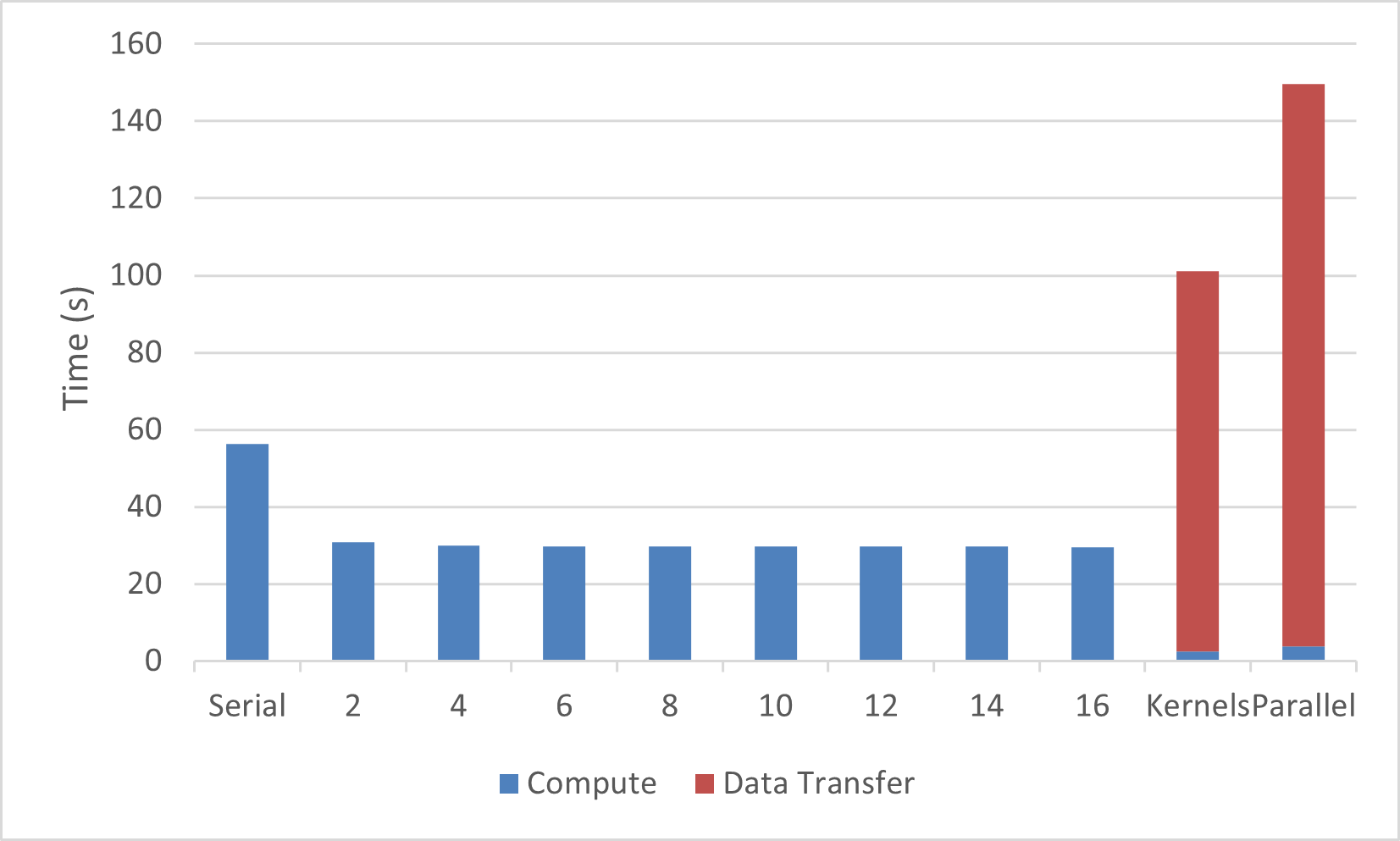
The performance of this improves as more CPU threads are added to the calculation,
however, since the code is memory-bound the performance benefit of adding
additional threads quickly diminishes. Also, the OpenACC versions perform poorly
compared to the CPU
baseline. Both the OpenACC kernels and parallel loop versions perform
worse than the serial CPU baseline. It is also clear that the parallel loop version
spends significantly more time in data transfer than the kernels version.
Further performance analysis is necessary to
identify the source of this slowdown. This analysis has already been applied to
the graph above, which breaks down time spent
computing the solution and copying data to and from the accelerator.
A variety of tools are available for performing this analysis, but since this
case study was compiled for an NVIDIA GPU, NVIDIA Nsight Systems will be
used to understand the application peformance. The screenshot in figure 3.2
shows Nsight Systems profile for 2 iterations of the convergence loop in
the parallel loop version of the code.
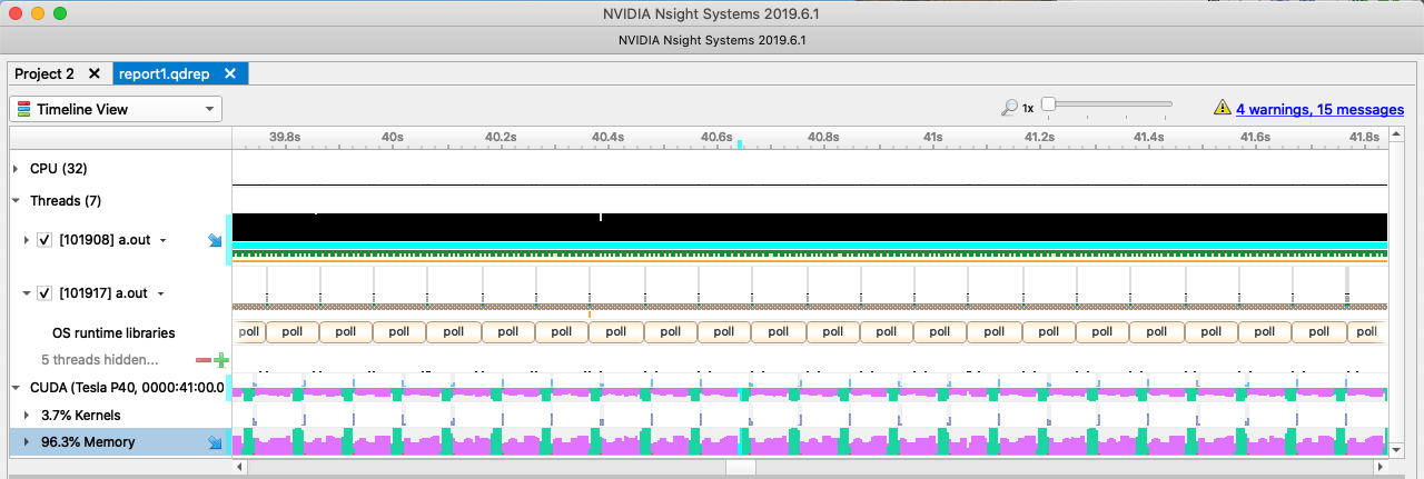
Since the test machine has two distinct memory spaces, one for the CPU and one
for the GPU, it’s necessary to copy data between the two memories. In this
screenshot, the tool represents data transfers using the tan colored boxes in the
two MemCpy rows and the computation time in the green and purple boxes in the
rows below Compute. It should be obvious from the timeline displayed that
significantly more time is being spent copying data to and from the
accelerator before and after each compute kernel than actually computing on the
device. In fact, the majority of the time is spent either in memory copies or
in overhead incurred by the runtime scheduling memory copeis. In the next
chapter we will fix this inefficiency, but first, why does the kernels
version outperform the parallel loop version?
When an OpenACC compiler parallelizes a region of code it must analyze the data
that is needed within that region and copy it to and from the accelerator if
necessary. This analysis is done at a per-region level and will typically
default to copying arrays used on the accelerator both to and from the device
at the beginning and end of the region, respectively. Since the parallel loop
version has two compute regions, as opposed to only one in the kernels
version, data is copied back and forth between the two regions. As a result,
the copy and overhead times are roughly twice that of the kernels region,
although the compute kernel times are roughly the same.